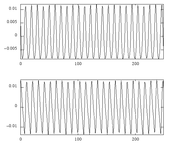
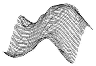
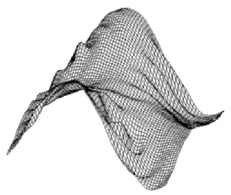
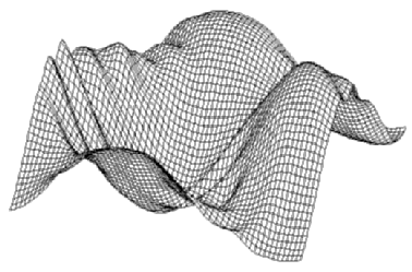
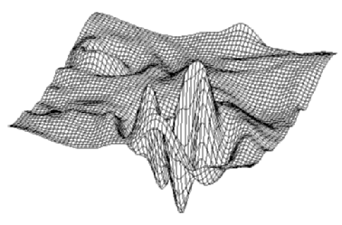
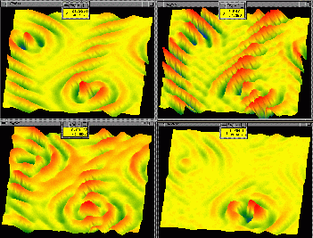
KLTOOL: A Mathematical Tool for Analyzing Spatiotemporal Data

Randy W. Heiland
Arizona State University, Dept of Mathematics, Dec. 1992

1. Introduction
2. Spatiotemporal Data
3. Dynamical Systems Concepts
4. Karhunen-Loève Decomposition
5. Overview of kltool
6. Examples
7. Future Directions
8. Summary
Bibliography
Appendix: Galërkin Projection for Kuramoto-Sivashinsky PDE

1. Introduction

The quantitative analysis of low-dimensional chaotic dynamical systems has been an active area of research for many years. Up until now, most work has concentrated on the analysis of time series data from laboratory experiments and numerical simulations. Examples include Rayleigh-Bénard convection, Couette-Taylor fluid flow, and the Belousov-Zhabotinskii chemical reaction [Libchaber, Fauve & Laroche '83], [Roux '83] and [Swinney '84].

The key idea is to reconstruct a representation of the underlying attractor from the time series. (The time-delay embedding method [Takens '81] is one popular approach). Given the reconstructed attractor, it is possible to estimate various properties of the dynamics - Lyapunov exponents and an attractor's dimension, for example. Local approximations of the dynamics make it possible to reduce noise in the original time series and to make short-term predictions of the system's behavior. [Kostelich & Yorke '90] and [Sugihara & May '90].

In contrast, methods for the analysis of spatiotemporal data are not as well developed. This thesis describes a computer-aided tool, called kltool, which operates on spatiotemporal data from nonlinear systems. Its primary function is to analyze the data and extract a set of basic building blocks - the eigenfunctions of the dataset. These eigenfunctions are optimal, in a certain least-squares sense, and they can reveal coherent spatial structures within the data. It is then possible to reconstruct an approximation to the data using these eigenfunctions. In addition to providing these analytic and synthetic modes of operation, kltool has other capabilities which offer insight into dynamical models for the data.

Although the underlying mathematical analysis is well known, there has not been an interactive software package to apply it to a given dataset. Kltool is intended to be an easy-to-use, general-purpose software package for nonspecialists. In addition to describing this software, we present some new and interesting results obtained during the tool's development.

In the next Chapter, we discuss further the spatiotemporal data to be analyzed. In Chapter 3, dynamical systems and related concepts are introduced. Chapter 4 describes the mathematical details of the Karhunen-Loève (K-L) decomposition - the analytic tool to be applied to a given dataset. Kltool, which incorporates the K-L algorithm with accompanying software, will be explained in Chapter 5. We present some results of kltool's analysis of different datasets in Chapter 6. Chapter 7 offers a few thoughts on future directions and we summarize in Chapter 8.

2. Spatiotemporal Data

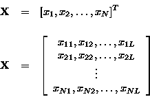
The type of data we wish to analyze are generated by some nonlinear system which evolves in time and which is spatially inhomogeneous. We assume a spatial vector, ${\bf X}$, is obtained at discrete time values, t_i, providing a set of spatiotemporal data: $\{{\bf X}_i\}_{i=1}^M$. The components of ${\bf X}$ correspond to scalar measurements taken at fixed points in space. We allow for the visualization of one- or two-dimensional spatial vectors:

Two common methods of obtaining such spatiotemporal data are from laboratory experiments and numerical simulations of a mathematical model - typically a partial differential equation (PDE).

The problem we address is: can this complex set of data be understood and explained in some relatively simple manner? It would seem to be possible if the complexity is generated by the temporal evolution of only a few spatial structures.

A standard approach in analyzing such data is to perform a Fourier decomposition. One would hope that only a few dominant peaks appear in a power spectrum of the spatial modes, suggesting relatively simple spatial structures. However, it may be that a coherent spatial structure is composed of many Fourier modes and a Fourier analysis would not be the best approach.

The decomposition used in this thesis, and discussed further in Chapter 4, can compute coherent spatial structures directly. Furthermore, the structures will be optimal (in a least-squares sense) for a given dataset. Once the primary spatial structures are known, we will try to explain their temporal evolution within the framework of dynamical systems theory. The key concepts of this theory will be presented in the next chapter. However, as a prelude, we offer the following thought.

A primary objective in applying dynamical systems theory to a nonlinear system is to understand the long-term (asymptotic) behavior of the system in a qualitative way. If the system is sufficiently complex, it is unlikely that one can make any quantitative predictions about the system. However, if it is possible to reduce the number of degrees of freedom inherent in the system then certain qualitative descriptions may be possible.

Consider a PDE as a nonlinear system. One could think of such a system as having ultimate complexity - by virtue of having infinitely many degrees of freedom. It is known that the solution of many PDEs can be expanded in an infinite set of Fourier modes [Strang '86]. However, for certain dissipative PDEs, the theory of attracting sets and inertial manifolds guarantee that these systems are actually finite dimensional. See [Ruelle '89] and [Jolly, Kevrekidis & Titi '90] for examples. In fact, numerical simulations of certain PDEs suggest that they have relatively low-dimensional attractors. It is data coming from such low-dimensional systems, either PDEs or laboratory experiments, with which this thesis is primarily concerned.

3. Dynamical Systems Concepts

In this chapter we present a few key concepts from dynamical systems theory. Within this mathematical theory, we hope to gain some understanding of nonlinear systems by examining their spatiotemporal data. An underlying assumption throughout this chapter is that the temporal dynamics of the systems being studied has relatively few degrees of freedom - on the order of ten or less.

A dynamical system is a way of describing the state of some system as it evolves in time. We illustrate via examples and simultaneously introduce related concepts and terminology.

Dynamical systems are commonly described by ordinary differential equations (ODEs) of the form:

$$\frac{d{\bf x}}{dt} = {\bf f}({\bf x},t;\mu)$$ (3.1)

with the dependent variables ${\bf x} \in I\!\!R^n$, the independent variable $t \in I\!\!R$, and possible free parameters $\mu \in I\!\!R^m$. The space of dependent variables is called the phase space (or state space) of a dynamical system.

The extensive theory of differential equations has an important role in the study of dynamical systems. For questions concerning the existence and uniqueness of solutions to (3.1), as well as other theoretical issues, see [Waltman '86]. When one tries to understand the asymptotic dynamics of differential equations, it is assumed that enough time has elapsed so that all transient behavior has died out.

We now describe how the study of dynamical systems makes use of geometric concepts. Since geometric descriptions are usually more intuitive than algebraic ones, the ideas are more easily grasped.

Every system of the form (3.1) implies a related vector field. The idea is simple. To each point in the phase space, we assign an instantaneous velocity vector obtained from the right-hand side of the system. A solution (also, orbit or trajectory) of (3.1) is a curve, ${\bf x}(t): I\!\!R\rightarrow I\!\!R^n$, whose tangent vector at any given t is the vector ${\bf f(x)}$ (at the point ${\bf x}$). Hence, we can compute a solution by integrating the right-hand side of the system. A solution, ${\bf x}(t)$, will depend on an initial condition, ${\bf x}_0$, and on the free parameters $\mu$.

We illustrate with a simple example. Consider the 2D autonomous¹, linear system:

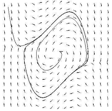
The vector field and a solution of (3.2) are shown in Figure 3.1.

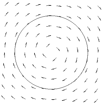
Figure 3.1 Vector field and a solution of (3.2).

For system (3.2), we see that all solutions are periodic. For any ${\bf x}_0 \neq (0,0)$, ${\bf x}(t)$ rotates forever about the origin. The origin is a fixed point (also critical point or equilibrium). Any solution starting at a fixed point will remain there. The particular type of fixed point in this example is called a center.

To find all fixed points of a system, one solves for the zeros of the system:

The study of dynamical systems has a primary goal - to understand the asymptotic (long-term) behavior of its solutions in a qualitative way. For example, solutions might: (1) approach some fixed point, (2) ``blow up'' after some finite time, (3) approach some periodic solution, or (4) follow some other complicated motion.

Typically, solutions of a system will undergo qualitative changes as one of the system's free parameters, ${\mu}_j$, is varied. Such a parameter is called a bifurcation parameter. Understanding these qualitative changes in the geometry of solutions in phase space is the subject of bifurcation theory [Wiggins '90].

Minor algebraic modifications to (3.2) lead to qualitatively different solution structures in phase space. For a slightly more complicated example, consider the coupled linear 2D system:

$$\begin{eqnarray*}{\dot x} &=& -x + 2y \\ {\dot y} &=& -2x - y \end{eqnarray*}$$

This system results in the fixed point at the origin to become a global attractor. The fixed point is called a sink. The vector field and a spiraling solution toward the origin are shown in Figure 3.2.

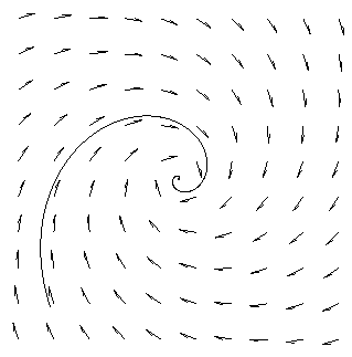
Figure 3.2 Vector field with a sink at (0,0).

The origin, still a fixed point, is repelling in the system:

$$\begin{eqnarray*}{\dot x} &=& x - 2y \\ {\dot y} &=& 2x + y \end{eqnarray*}$$

This type of fixed point is called a source. The vector field and an outward spiraling solution are shown in Figure 3.3.

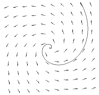
Figure 3.3 Vector field with a source at (0,0).

An example of a fixed point being both attracting (stable) and repelling (unstable) - in different directions, is given by the system:

$$\begin{eqnarray*}{\dot x} &=& -x + 2y \\ {\dot y} &=& 2x + y \end{eqnarray*}$$

Here, the fixed point at the origin is called a saddle. The vector field is shown in Figure 3.4.

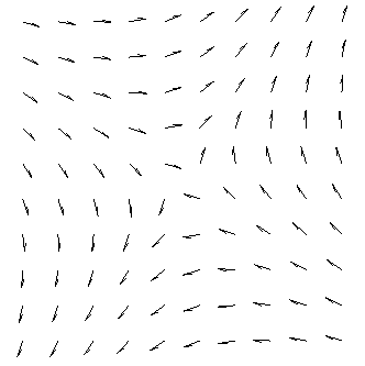
Figure 3.4 Vector field with a saddle at (0,0).

From the theory of ODEs, we know that the stability of fixed points of linear systems can be determined from the eigenvalues of the coefficient matrix of the right-hand side. In the above systems, the sink is asymptotically stable, the center is stable (but not asymptotically), and the source and saddle are unstable.

Nonlinear systems are more likely to be used as models for real-life systems. They are more complex than linear systems and give rise to more interesting phase space structures than fixed points. For example, in 2D (and higher) nonlinear systems, one can find limit cycles. A limit cycle is a closed, periodic orbit which can be either attracting or repelling. As an example, the following nonlinear system contains an attracting limit cycle. The system is a model for electrical circuits whose resistive properties change according to the supplied current. It is known as the van der Pol system:

$$\begin{eqnarray*}{\dot x} &=& y - (x^3 - \mu x) \\ {\dot y} &=& -x \end{eqnarray*}$$

The parameter $\mu$ is a bifurcation parameter. When $\mu < 0$, the origin is a global attractor. When $\mu > 0$, the origin loses stability, becoming a repellor, and an attracting limit cycle is created. The point at which this happens is known as a Hopf bifurcation point. A limit cycle of this system, for $\mu = 1$, is shown in Figure 3.5. A solution starting near the origin is attracted outward to the limit cycle, whereas a solution starting outside the limit cycle is attracted inward to it. The asymptotic solutions, x(t) and y(t), would be sinusoidal as plotted in Figure 3.6.

Figure 3.5 An attracting limit cycle.

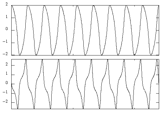
Figure 3.6 x(t), y(t) of limit cycle.

The Poincaré-Bendixson theorem is useful for guaranteeing the existence of a limit cycle in 2D autonomous systems of ODEs [Hirsch & Smale '74]. The stability of fixed points becomes a local property for nonlinear systems. One must linearize the system about a fixed point to determine that fixed point's stability. See [Waltman '86] for this important theory.

There are other closed, but nonperiodic, orbits which occur in phase space. A homoclinic orbit is one which leaves the neighborhood of a fixed point along an unstable direction and loops back on itself along a stable direction. A heteroclinic orbit connects two (or more) different fixed points together via their stable and unstable manifolds as illustrated in Figure 3.7.

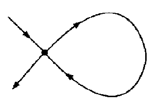
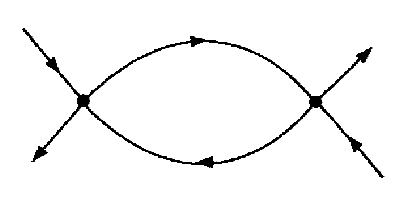
Figure 3.7 A homoclinic and heteroclinic orbit.

So that one does not conclude $I\!\!R^n$ is the only possible phase space, we describe a classic example of a dynamical system - the pendulum. This physical system is illustrated in Figure 3.8. It consists of a bob

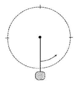
Figure 3.8 The simple pendulum.

attached to a rigid rod which rotates around an axis. The state of the system is most naturally described by it phase and angular velocity: $\theta$ and $\omega={\dot \theta}$, with $0 \leq \theta \leq 2\pi$.

The dynamics are given by the system:

$$\begin{eqnarray*}{\dot \theta} &=& \omega \\ {\dot \omega} &=& -\frac{1}{l}sin\theta - \frac{k}{m}\omega \end{eqnarray*}$$

The phase space is therefore an infinite cylinder: $S^1\times I\!\!R$. For plotting convenience, however, this cylinder can be mapped into $I\!\!R^2$ with $\theta$ being $2\pi$-periodic along the horizontal axis. Solutions in this phase space for the undamped system (k=0) are shown in Figure 3.9 and for the damped system (k>0) in Figure 3.10.

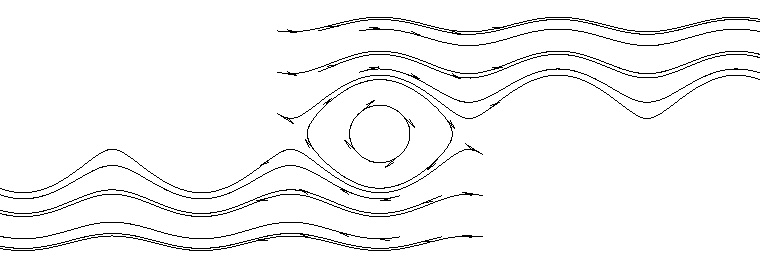
Figure 3.9 Solutions of the undamped pendulum.

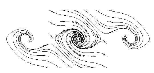
Figure 3.10 Solutions of the damped pendulum.

The base of each vector in the vector field serves as an initial value for a solution. In the undamped system, the position $\theta=0$ is locally a center. This means that for small enough angular velocity, $\omega$, the pendulum will swing back and forth about $\theta=0$ without ever making a full revolution. However, for too large angular velocity, the pendulum will forever revolve about its axis in only one direction. In the damped system, $\theta=0$ becomes a sink (locally) and any nearby orbits get attracted to this fixed point. The point $\theta=\pi$ is a saddle. A homoclinic orbit would leave from and return to this point.

Going to three-dimensional systems, even more interesting dynamics and geometric structures occur in phase space. We illustrate with a well known system given by [Lorenz '63]:

$$\begin{eqnarray*}{\dot x} &=& \sigma(y - x) \\ {\dot y} &=& {\rho}x - y - xz \\ {\dot z} &=& {\beta}z + xy \end{eqnarray*}$$

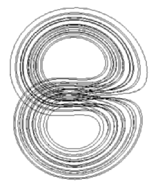
This system is an over-simplified model for convection. It is also a model for a perfectly tuned two-level laser [Newell & Moloney '92]. The dynamics and bifurcations of the Lorenz system are discussed in [Sparrow '82]. For particular values of the bifurcation parameters, $\sigma,\rho$, and $\beta$, an interesting attractor appears in phase space. Unlike a fixed point or a limit cycle, this attractor has a more complicated geometric structure. It is a three-dimensional ``figure-8'' shape. However, the attractor is not a closed orbit. Rather, it has some ``thickness''. We show a solution captured within this attracting structure in Figure 3.11. This idea of having a deterministic system which results in complex, yet coherent, dynamics is the backdrop for chaos theory [Wiggins '88] which has been popularized in [Gleick '87].

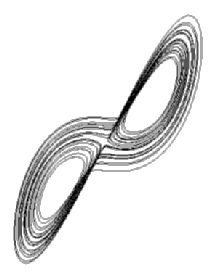
Figure 3.11 Lorenz attractor projected onto the xy plane (top) and yz plane (bottom).

It was stated earlier that a primary goal of studying dynamical systems is to understand the long-term dynamics in a qualitative way. The Lorenz attractor offers a good example. We know that for certain parameter values of the system, solutions will asymptotically remain confined to the subspace in which the attractor lies. This raises another key concept in dynamical systems theory - the dimension of attractors. It is for this topic that dynamical systems requires the notion of fractals and fractional dimensions [Barnsley '88] and [Farmer, Ott & Yorke '83].

Being able to compute the dimension of an attractor and to construct the attractor, using empirical data from a dynamical system, has been an active area of research [Broomhead & King '85], [Sauer, Yorke & Casdagli '91], [Kostelich '92], and [Gibson, Farmer, Casdagli & Eubank '92]. These methods typically operate on a time series of some scalar measurement of the system as mentioned in Chapter 1. This is inherently different from the analysis treated in this thesis which deals with spatiotemporal data, as discussed in Chapter 2.

In conclusion, we want to bridge the gap between the low-dimensional dynamical systems as presented in this chapter and the infinite-dimensional PDEs as discussed in Chapter 2. This is done via a Galërkin projection. Assuming the solution to a PDE can be approximated by the expansion:

$$\begin{eqnarray*}u(x,t) \approx \sum_{i=1}^N a_i(t)\phi_i(x) \end{eqnarray*}$$

where the $\phi_i$ are known spatial structures, then the time-dependent coefficients, a_i(t), are obtained as solutions of an N-dimensional system of ODEs, known as a Galërkin projection:

$$\begin{eqnarray*}{\dot {\bf a}} = {\bf f}({\bf a}) \end{eqnarray*}$$

We then need to make analogous classifications of a PDE's asymptotic dynamics with those of a system of ODEs as presented in this chapter. A fixed point corresponds to a stable spatial structure of a PDE. A limit cycle corresponds to some oscillating spatial structure, for example, either a standing wave or a travelling wave. And chaotic (``strange'') attractors which are low-dimensional should correspond to spatiotemporal complexity generated by the temporal evolution of only a few coherent spatial structures.

This chapter has presented some basic definitions and concepts of dynamical systems. For a visual and intuitive introduction, see [Abraham & Shaw '84]. A graphical environment for experimenting with dynamical systems on a personal computer can be found in [Koçak '86]. Other computer packages which offer a more sophisticated analysis of dynamical systems are [Guckenheimer & Kim '90] and [Yorke '90]. For a thorough and mathematically rigorous treatment of this subject, see [Guckenheimer & Holmes '83] and [Wiggins '90].

4. Karhunen-Loève Decomposition

The method of analysis at the core of this thesis appears in various guises and is known by different names - depending on the area of application. In image processing, it is known as the Hotelling transform [Gonzalez & Wintz '87]. In pattern recognition, the name principal component analysis is commonplace. Both application areas typically analyze an ensemble of static data. For example, consider an image from a satellite's camera. The same image will be transmitted repeatedly, but each version will be slightly noise-contaminated due to Earth's atmosphere. A subsequent analysis is performed to remove, or at least reduce, the noise.

The method is also known as the Karhunen-Loève (K-L) decomposition. However, in the context of this thesis, the data to be analyzed will be temporally evolving rather than being an ensemble.

Another name for this method is proper orthogonal decomposition (POD). [Lumley '67] proposed that the method be used in fluid flow analysis. He suggested that it could provide an unbiased identification of coherent structures in turbulent flow. See [Aubry, Holmes, Lumley & Stone '88] for an application.

Regardless of the name and the application, the method is essentially the same. It is based on second-order statistical properties [Loève '55] which result in a set of optimal eigenfunctions. We now present the theory behind the decomposition.

First, we assume data to be a set of (real) random vectors:

$$\begin{eqnarray*}\{{\bf X}_i\}_{i=1}^M \end{eqnarray*}$$

where ${\bf X} = [x_1,x_2, \ldots ,x_N]^T$. In the classical theory from statistical pattern recognition [Fukunaga '90], one would then need to characterize each random vector with a probability density function. This would be used to define, via integration, the mean of a random vector. Finally, the covariance matrix, indicating the dispersion of the vectors' distribution, could be calculated. It is this matrix which provides the information that we want. Specifically, we wish to know its eigenvalues and eigenvectors.

These theoretical calculations are approximated in actual computations from the given set of vectors. The mean is computed as:

$$\begin{eqnarray*}\overline{{\bf X}} = \frac{1}{M} \sum_{i=1}^M {\bf X}_i \end{eqnarray*}$$

For convenience, we then compute an additional sequence of vectors which have zero mean:

$$\begin{eqnarray*}\hat{{\bf X}}_i = {\bf X}_i - \overline{{\bf X}},\hspace*{0.5in} i=1,\ldots,M \end{eqnarray*}$$

The $\hat{{\bf X}}_i$ are called the caricature vectors.

The covariance matrix is then approximated by:

$$\begin{eqnarray*}{\bf C} = \frac{1}{M} \sum_{i=1}^M \hat{{\bf X}}_i \hat{{\bf X}}_i^T \end{eqnarray*}$$

We point out that the covariance matrix is an $N \times N$matrix, where N is the spatial resolution of a vector. For large N, this matrix can become too large for practical computation. However, by using the method of snapshots, as described by [Sirovich '87a], the computation becomes more tractable. Using this method, the covariance matrix becomes:

$$\begin{eqnarray*}{\bf C}_{ij} = \langle \hat{{\bf X}}_i,\hat{{\bf X}}_j \rangle , \hspace*{0.5in} i,j=1,\ldots,M \end{eqnarray*}$$

where $\langle\cdot,\cdot\rangle$ denotes the usual Euclidean inner product. The matrix is now $M \times M$ instead of $N \times N$ and, assuming M<N, we can compute its eigenvalues and eigenvectors more easily.

Since the covariance matrix is symmetric, we know that its eigenvalues, $\lambda_i$, are nonnegative and its eigenvectors, $\phi_i$, $i=1, \ldots, M$, form a complete orthogonal set [Strang '76].

The orthogonal eigenfunctions of the data are defined as:

$$\begin{eqnarray*}{\Psi}^{[k]} = \sum_{i=1}^M {\phi}_i^{[k]} \hat{\bf X}_i, \hspace*{0.5in} k=1,\ldots,M \end{eqnarray*}$$

where ${\phi}_i^{[k]}$ is the i-th component of the k-th eigenvector. Lumley refers to these eigenfunctions as coherent structures of the data. Whether or not they would appear as spatial structures in a laboratory experiment is questionable [Sirovich '87b]. Nevertheless, there is cause to believe that they will be present at least indirectly. Perhaps an actual structure will consist of a linear combination of eigenfunctions.

A characterization of the eigenfunctions is that they form an optimal basis for the expansion of a spatiotemporal dataset:

$$\begin{eqnarray*}u(x,t) \approx \sum_{i=1}^K a_i(t)\Psi_i(x) \end{eqnarray*}$$

by minimizing the L² norm of the error.

The ``energy'' of the data is defined as being the sum of the eigenvalues of the covariance matrix:

$$\begin{eqnarray*}E = \sum_{i=1}^M {\lambda}_i \end{eqnarray*}$$

To each eigenfunction we assign an energy percentage based on the eigenfunction's associated eigenvalue:

$$\begin{eqnarray*}E_k = \frac{\lambda_k}{E} \end{eqnarray*}$$

Assuming the eigenvalues are sorted largest to smallest, we have an ordering of the eigenfunctions from most to least energetic .

Finally, we can reconstruct any sample vector using the eigenfunctions:

$$\begin{eqnarray*}{\bf X} = \overline{{\bf X}} + \sum_{i=1}^M{a_i {\Psi}^{[i]}} \end{eqnarray*}$$

where the coefficients are computed from the projection of the sample vector onto an eigenfunction:

$$\begin{eqnarray*}a_i = \left( \frac{\hat{\bf X} \cdot {\Psi}^{[i]}} {{\Psi}^{[i]} \cdot {\Psi}^{[i]}} \right) \end{eqnarray*}$$

Using only the first K (K<M) most energetic eigenfunctions, we can construct an approximation to the data:

$$\begin{eqnarray*}{\bf X} \approx \overline{{\bf X}} + \sum_{i=1}^K{a_i {\Psi}^{[i]}} \end{eqnarray*}$$

As a final note, we mention that the results of the above K-L decomposition can also be obtained via singular value decomposition (SVD). See [Strang '76] for an introduction to SVD. Using this method, one would not compute the $M \times M$ covariance matrix. Instead, an $N \times M$ rectangular matrix is generated:

$$\begin{eqnarray*}\left[ \hat{\bf X}_1,\hat{\bf X}_2, \ldots ,\hat{\bf X}_M \right] \end{eqnarray*}$$

The singular values, ${\sigma}_i$, $i=1, \ldots, M$ (assuming M<N) and singular vectors of this matrix are then computed. Using the fact that ${\sigma}_i^2 = \lambda_i$, the computations would proceed as above. An application and discussion of the SVD method for a PDE modeling fluid motion can be found in [Newell, Rand & Russell '88]. A comparison of SVD and K-L, in terms of numerical accuracy, is discussed in [Mees, Rapp & Jennings '87].

5. Overview of kltool

We now describe the computer implementation of the Karhunen-Loève (K-L) decomposition as explained in the previous chapter. First, we discuss some implementation issues and present an overview of capabilities of kltool. We then describe specific applications of kltool using examples in Chapter 6.

5.1. Implementation

Pragmatic considerations determined how kltool is implemented. We wanted hardware which could render high-quality graphics and perform reasonably fast computations. Also, since we wanted to make the tool available to others, selecting a widely available platform was important. The Silicon Graphics Personal Iris was selected for the initial implementation primarily because of its high-quality 3D graphics.

On the software side, the tool is implemented in the C programming language. All graphics are performed using the Graphics Library, a set of graphics routines available on Silicon Graphics workstations. The numerical decomposition routines are obtained from public domain software libraries.

5.2. Functionality

The functionality of kltool generally adheres to the current trend of workstation applications: interacting with the user via popup menus and dialog boxes and displaying results in multiple windows on the screen. These nontrivial issues are discussed in [Shneiderman '80].

A schematic overview of kltool's functionality is depicted in Figure 5.1. We briefly describe the function of each operation:

Figure 5.1 Overview of kltool.

Input

Reads the dataset of vectors (or some subset thereof). The user specifies the spatial dimension of the vector (currently, only one- or two-dimensional vectors can be visualized) and the vector resolution. Examples of vectors might be 2D images from a laboratory experiment, or discretized solutions of a PDE.

Visualize

Allows viewing of the data. One can select from a list of viewing modes: wireframe or colored surface, scan or landscape.

Select

Interactive selection of a subset of the data. This feature can be quite important. A dataset cannot be generated arbitrarily but must contain the appropriate dynamics for the analysis to be successful. This point will become more clear in the examples.

Mean

Compute and display the temporal average of the time series of vectors.

Covariance

Compute the covariance matrix, ${\bf C}$.

Decompose

Perform K-L decomposition on ${\bf C}$. (Alternatively, perform singular value decomposition). This results in a bar-chart display of energy percentages of the eigenvalues (with a default cumulative of 95%). The empirical eigenfunctions are then computed and displayed.

Coefficients

Compute and display the time series coefficients of the data projected onto an eigenfunction.

Reconstruct

Compute and display an approximation to the original data using K eigenfunctions.

Error

Compute and display the absolute error between the data and its approximation.

Galërkin Projection

Generate a Galërkin projection, a system of ODEs, for a PDE using K eigenfunctions. One must provide the PDE in a predefined syntax. kltool's algorithm scans the symbolic PDE, searches for differentiation operators, $d(u,x,\cdot)$, and performs the appropriate substitution and differentiation of K eigenfunctions. An example is provided in Section 6.1.1.

These functions are implemented in the software in a modular style. This allows for errors to be easily traced and for new functionality to be easily incorporated. For a more thorough description of the tool's operation, see [Armbruster & Heiland '92].

6. Examples

We present four different examples of spatiotemporal data and their resulting analyses using kltool. In the first example, data from a numerical simulation of a partial differential equation (PDE) is analyzed. In the second example, we examine data from a fluid flow experiment. The third example provides a recent analysis of dynamics from a PDE simulation of fluid flow. In the last example, we analyze video data from an experiment involving flame dynamics.

It is regrettable that the true dynamics found in these examples cannot be better presented on paper. A more natural medium would be video. Nevertheless, we provide a depiction of the dynamics via landscape plots (for 1D spatial vectors) and a set of frames (for 2D vectors). We note, however, that the landscape plots represent only an appropriately sampled subset of the entire dataset. This is done to make the plots more legible.

6.1. Kuramoto-Sivashinsky Equation

As an early test case for kltool, we chose a PDE which had previously been studied using K-L analysis [Kirby & Armbruster '91]. The PDE is known as the Kuramoto-Sivashinsky (K-S) equation:

$$\begin{eqnarray*}u_t + 4u_{xxxx} + \alpha(u_{xx} + \frac{1}{2}(u_x)^2) = 0,\hspace*{0.5in} 0\leq{x}\leq{2\pi} \end{eqnarray*}$$

We impose periodic boundary conditions: $u(0,t)=u(2\pi,t)$.

This equation is used as a model for flame fronts and thin viscous fluid films, among other phenomena. Much of its spatiotemporal dynamics are known, through an exhaustive numerical study, and described in [Hyman, Nicolaenko & Zaleski '86]. As the bifurcation parameter, $\alpha$, increases, the dynamics exhibit a variety of interesting behavior, including: fixed points, traveling waves, beating waves, homoclinic and heteroclinic orbits, and chaos.

For the purpose of our analysis, we chose two values for $\alpha$which produce distinctive dynamics.

6.1.1. Homoclinic Cycle

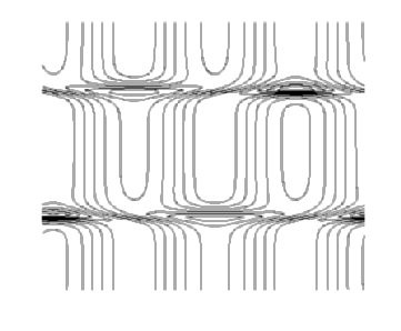
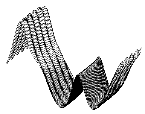
For =17.75, the K-S equation is known to have a homoclinic cycle. In fact, these dynamics have been explained in an analytic framework [Armbruster, Guckenheimer & Holmes '89] and [Kevrekidis, Nicolaenko & Scovel '90]. To verify that kltool could correctly analyze this situation, we numerically computed a time series of 1D spatial solution vectors as input. The solutions were discretized at a resolution of 256 discrete points over the $2\pi$ domain. We computed 400 snapshots in time. This dataset is depicted in Figures 6.1 and 6.2 and is characterized by two bursts.

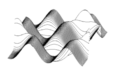
Figure 6.1 K-S (=17.75) dataset landscape plot

Figure 6.2 K-S (=17.75) dataset contour plot

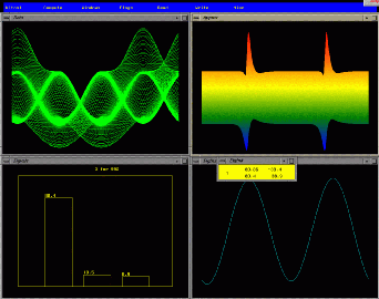
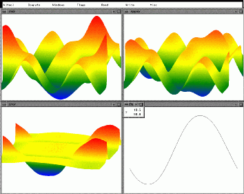
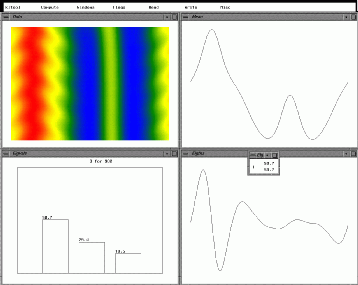
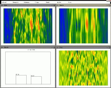
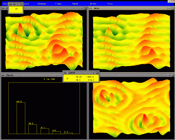
The K-L analysis results are shown in Figures 6.3 and 6.4. Figure 6.3 shows a screen image from kltool. In the upper-left window, the dataset is plotted in landscape mode. The view is from the front, meaning that the spatial coordinate is horizontal and the temporal snapshots are going ``into'' the screen. The vertical direction measures the amplitude of the solutions, u(x,t). In the upper-right, the dataset is displayed as a color-coded surface from the side view, meaning the horizontal axis is now t. This view highlights the bursting behavior of the data. In the lower-left window, a bar-chart indicates the energy percentages of the first three eigenfunctions. Recall that kltool, by default, will compute enough eigenfunctions for at least 95% of the total energy. We see that the first eigenfunction (K-L mode), $\Psi_1$, has most ($\approx$ 80%) of the total energy. In the lower-right window, $\Psi_1$ is plotted (scaled independently of the dataset windows).

Figure 6.3 K-S (=17.75) data from front (x horiz)(u-l), side (t horiz)(u-r), energy %s(l-l), $\Psi_1$(l-r).
(click on image for 1278x1022 enlargement)

Referring back to Figure 6.1, we see that $\Psi_1$ represents the state of the system before the first burst and after the second burst. There is a different state between bursts. Therefore, in phase space concepts, we have a heteroclinic orbit: we leave one unstable fixed point, go to another, and return to the original. It so happens, however, that $\Psi_1$ also represents the steady state (fixed point) found between bursts. It is simply a $\pi/2$  phase-shifted copy of the other steady state. Typically, such fixed points would be structurally unstable and would not occur in simulations. However, for certain symmetric systems, of which this system is an example, theory can explain why such fixed points are structurally stable. The special type of heteroclinic orbit, involving phase-shifted fixed points, is called a homoclinic cycle.

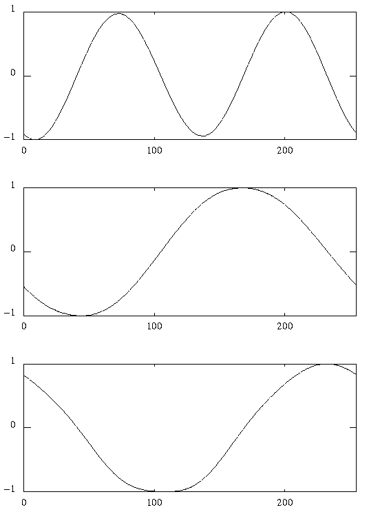
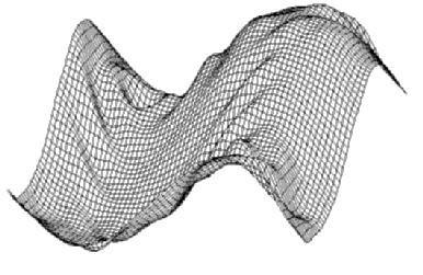
Figure 6.4 shows the first three eigenfunctions: $\Psi_1,\Psi_2,\Psi_3$(each mapped into the amplitude range [-1,1]). We perform a reconstruction of the dataset using only $\Psi_1$ and $\Psi_2$.

Figure 6.4 K-S (=17.75) , , and .

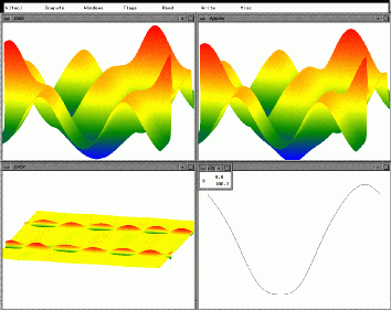
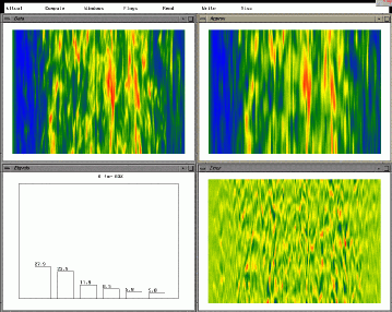
Figure 6.5 shows the original data (upper-left), the reconstruction (upper-right), and the absolute error (lower-left). All three plots are drawn to the same scale. Notice that the error is most significant during the bursts, that is, during the excursion between steady states.

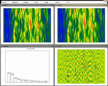
In Figure 6.6, we show a reconstruction of the data using $\Psi_1,\Psi_2,$and $\Psi_3$. Notice that the error is now much smaller than before. This indicates that $\Psi_3$ is involved in the bursts, as one might have suspected.

Figure 6.5 K-S (=17.75) dataset(u-l), reconstruction with , (u-r), error(l-l), (l-r).
(click on image for 1278x1022 enlargement)

Figure 6.6 K-S (=17.75) dataset(u-l), reconstruction with , ,(u-r), error(l-l), (l-r).
(click on image for 1278x1022 enlargement)

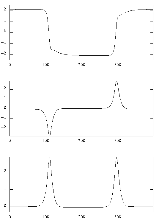
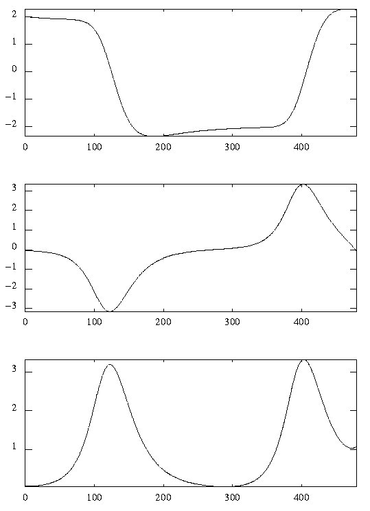
Figure 6.7 shows the coefficients of $\Psi_1,\Psi_2,$ and $\Psi_3$ as a time series. This confirms the analysis results: $\Psi_1$ represents the unstable fixed points (differing by a phase shift); $\Psi_2$ and $\Psi_3$ are dormant near the fixed points, but get activated during the bursts.

Figure 6.7 K-S (=17.75) Coefficients of , , and .

We use this dataset as an example on which to perform a Galërkin projection. First, we express the solution of the PDE as a linear combination of time-dependent coefficients and spatial eigenfunctions, resulting in a K-L Galërkin expansion:

$$u(x,t) \approx \sum_{i=1}^K{a_i(t)\Psi_i(x)}$$ (6.1)

where K is the number of eigenfunctions chosen for the reconstruction.

The K-S PDE is then rewritten as:

$$u_t = -4u_{xxxx} - \alpha(u_{xx} + \frac{1}{2}(u_x)^2)$$ (6.2)

Plugging (6.1) into (6.2) and differentiating, we obtain:

$$\sum_{i=1}^K{{\dot a}_i\Psi_i} = -4\sum_{i=1}^K{{a_i}{\Psi_i}^{(4... ...a (\sum_{i=1}^K{{a_i}{\Psi_i}''} + \frac{1}{2}(\sum_{i=1}^K{{a_i}{\Psi_i}'})^2)$$ (6.3)

where ${\dot a}$ denotes differentiation with respect to t, $\Psi'$ is with respect to x, and for conciseness, the independent variables are omitted.

Now we describe how the K-L Galërkin projection is performed within kltool. We write each $\Psi_i$ as a Fourier expansion:

$$\begin{eqnarray*}\Psi_m = \sum_{k=-H}^H{{c_{k,m}}e^{ikx}} \end{eqnarray*}$$

(where H depends on the spatial discretization of $\Psi$) and recall the orthogonality condition of the $\{\Psi_i\}$:

$$\begin{eqnarray*}(\Psi_i,\Psi_j) = \left\{ \begin{array}{ll} 0 & $i$\space \neq $j$\space \\ C_i & $i=j$ \end{array} \right. \end{eqnarray*}$$

where C_i is a constant.

Multiplying (6.3) by $\Psi_j, j=1,\ldots,K$ and integrating from 0 to $2\pi$, we obtain a Galërkin projection, a system of ODEs, for the PDE. Appendix A shows the resulting system generated by kltool, using the first three K-L modes. This ODE system is then numerically integrated ² and the time series solutions are plotted in Figure 6.8.

Figure 6.8 K-S (=17.75) Galerkin projection time series solutions.

Comparing these solutions with the time series of Figure 6.7, we see the qualitative approximation that this synthesis offers. A primary reason for the ``smoothing out'' of the spikes in the time series plots is because $\Psi_1$ lacks a symmetric counterpart. By symmetrizing the eigenfunctions, we should obtain better results. It should be noted that cubic damping terms were added to the ODE system to prevent blow-up solutions, as suggested in [Kirby & Armbruster '91].

6.1.2. Strange Mode

We now analyze a dataset from the K-S PDE for =84.25. We take 200 solution snapshots in time. The dataset is depicted in Figure 6.9. We know from [Hyman, Nicolaenko & Zaleski '86] and [Kirby & Armbruster '92] what an analysis should produce. For =72, the PDE has a stable fixed point. The fixed point is shaped as a two-humped curve, one hump larger than the other, and is called a ``strange'' fixed point. At =83.75, this fixed point becomes unstable and undergoes a Hopf bifurcation. This results in an oscillation riding on top of the larger hump as we see in Figure 6.9.

Figure 6.9 K-S (=84.25) dataset landscape plot.

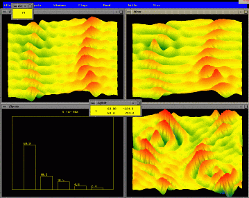
Figure 6.10 shows kltool's analysis of the given dataset. In the upper-left window, a color-coded surface of the data is viewed from the top. This produces a color-contour plot with a horizontal x-coordinate and vertical t-coordinate. The mean of the data, having the shape of the fixed point at =72, is plotted in the upper-right window. The energy percentages are plotted in the lower-left, showing that the first three eigenfunctions contain 98% of the total energy. In the lower-right window, the first eigenfunction, $\Psi_1$, is plotted. This clearly reveals the oscillation localized around the larger hump.

Figure 6.10 K-S (=84.25) color contours(u-l) mean(u-r), energy %s(l-l), (l-r).
(click on image for 1278x1022 enlargement)

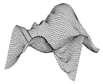
We note that the eigenfunctions as computed would indicate the dynamics of the data after the mean is subtracted. However, it is also possible to let kltool perform a K-L analysis without subtracting the mean. It seems to be an open research problem to determine whether the first eigenfunction for such a situation is in fact the mean. For this dataset at least, the first eigenfunction is essentially the mean of the data and it contains 99.4% of the total energy. The first three eigenfunctions are plotted in Figure 6.11.

Figure 6.11 K-S (=84.25) (=mean), , and .

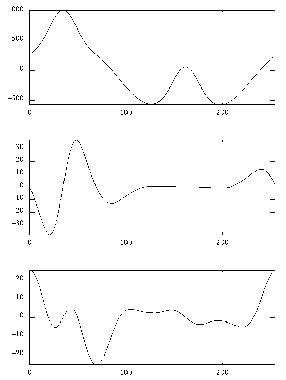
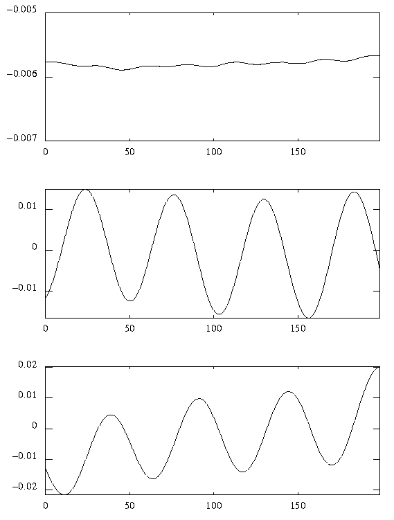
By projecting the data onto these eigenfunctions, we obtain the time series coefficients for $\Psi_1,\Psi_2,$ and $\Psi_3$ as shown in Figure 6.12. The time series for the coefficients of $\Psi_1$ is nearly constant and those of the remaining eigenfunctions are oscillatory. This suggests that the dynamics consist of a limit cycle encircling an unstable, yet dominant, fixed point. The limit cycle is essentially spanned by three K-L modes. Some recent research suggests that $\Psi_3$ may in fact be a travelling structure [Stone '92]. This would be believable judging from the upward slope of $\Psi_3$'s coefficients in Figure 6.12.

Figure 6.12 K-S (=84.25) coefficients of , , and .

6.2. Couette-Taylor Flow

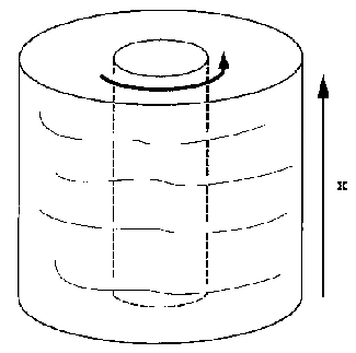
The Couette-Taylor experiment is widely known among fluid dynamicists. The apparatus consists of a cylindrical tank with a smaller, inner cylindrical tank. A fluid is contained between their two walls and the inner cylinder rotates - inducing a flow of the fluid. This flow has qualitatively different states, or flow patterns, depending on the rotation speed of the inner cylinder [DiPrima & Swinney '81]. Allowing both cylinders to rotate, either in the same or opposite direction, causes different flow patterns to form. Couette, a French scientist, was the first to experiment with this in the 1880's. In the 1920's, Taylor, a British mathematician, found some of the more interesting patterns. An enlightening, non-mathematical discussion of this experiment is found in [Stewart & Golubitsky '92].

For the purpose of our analysis, we were provided with data obtained in the following manner. The apparatus was photographed with a specially modified camera containing a charge-coupled device (CCD) array. A one-dimensional spatial vector of light intensity values in the azimuthal direction was recorded at regular time intervals, providing an indication of the system's flow pattern. An illustration of the experiment is shown in Figure 6.13.

Figure 6.13 Schematic illustration of Couette-Taylor experiment.

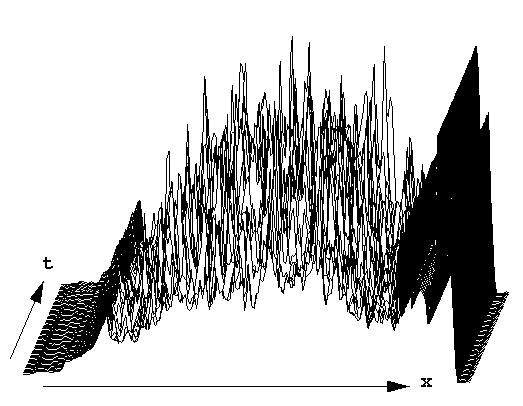
Figure 6.14 Couette-Taylor dataset.

The dataset consisted of 291 snapshot vectors, each with 891 components whose values were proportional to the light intensity. The dataset is depicted in Figure 6.14. One can see from this plot that near both ends of the spatial vectors, the amplitudes are constant in time. These values correspond to a boundary layer at the top and bottom of the Couette apparatus and are not relevant to the fluid behavior in the middle portion of the cylinder. Therefore, we make use of kltool's interactive data selection feature to remove the data near the boundaries. The resulting clipped vectors are then analyzed.

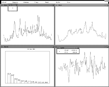
First, we show analysis results using only the first 50 snapshots of the dataset. Figure 6.15 shows the 31-st snapshot in the data window (upper-left), the mean of the dataset (upper-right), the $\Psi$ energy percentages (lower-left), indicating 12 are necessary for 95%, and $\Psi_1$ (lower-right). After scanning through the snapshots³, we observe that the data is quite ``noisy''. This contributes to an analysis which suggests the dynamics are not as low-dimensional as one might hope. The ratio of 12 eigenfunctions to 50 snapshots indicates high-dimensional phase space dynamics.

Figure 6.15 Couette-Taylor: snapshot(u-l) mean(u-r), energy %s(l-l), (l-r).
(click on image for 1278x1022 enlargement)

In spite of these discouraging results, we still perform a reconstruction of the data using the first K eigenfunctions. Figure 6.16 shows a color-contour plot of the original dataset (upper-left), a reconstruction using the first two eigenfunctions (K=2) (upper-right), and the absolute error (lower-right). Figure 6.17 shows a reconstruction with K=6 and Figure 6.18 shows a reconstruction with K=12. Notice that the successive error plots contain less coherent structure, indicating a better approximation with more eigenfunctions.

Figure 6.16 Couette-Taylor: dataset(u-l) reconstruction with , (u-r), energy %s(l-l), error(l-r).
(click on image for 1278x1022 enlargement)

Figure 6.17 Couette-Taylor: dataset(u-l) reconstruction with -(u-r), energy %s(l-l), error(l-r).
(click on image for 1278x1022 enlargement)

Figure 6.18 Couette-Taylor: dataset(u-l) reconstruction with -(u-r), energy %s(l-l), error(l-r).
(click on image for 1278x1022 enlargement)

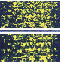
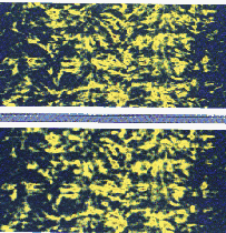
Next, we perform an analysis of the entire dataset, consisting of 291 snapshots. The results indicate that 46 eigenfunctions are necessary to capture 95% of the total energy. Figure 6.19 shows the original dataset (upper) and a reconstruction using only the first 10 eigenfunctions (lower). Figure 6.20 shows a reconstruction using the first 25. Depending on the desired goal, one might conclude that a resonable approximation can be obtained with fewer $\Psi_i$ than necessary for 95% of the energy. Certainly, fewer eigenfunctions are necessary to capture only the dominant (red) structures.

Figure 6.19 Couette-Taylor: entire dataset(top), reconstruction with - (bottom).
(click on image for 658x679 enlargement)

Figure 6.20 Couette-Taylor: entire dataset(top), reconstruction with - (bottom).
(click on image for 666x687 enlargement)

6.3. Kolmogorov Flow

This example, like the last, examines the topic of fluid flow. Here, we do so via a PDE numerical simulation.

The notion of turbulence in fluid flow is still not understood. There are, however, certain scenarios which seem to serve as forerunners to turbulence [Eckmann '81]. One such scenario involves intermittent bursting of certain measured quantitites. We analyze data of this type here. For a mathematical introduction to fluid flow, see [Chorin & Marsden '90]. A non-mathematical introduction to turbulence can be found in [Ruelle '91].

The PDE we consider is a version of the Navier-Stokes equation. The 2D Kolmogorov flow is the solution of the 2D incompressible Navier-Stokes equation subject to a force in the x-direction proportional to $\cos y$: $f=(\nu k_f^3 \cos k_f y,0)$. It was introduced by Kolmogorov in the late 1950's as an example on which to study transition to turbulence. For large enough viscosity $\nu$, the only stable flow is the plane parallel periodic shear flow $u_0 = ( k_f \cos k_f y,0)$, usually called the ``basic Kolmogorov flow''. The macroscopic Reynolds number of the basic flow is found to be $1/\nu$. This Reynolds number, Re, is used as a bifurcation parameter.

In a $2\pi$-periodic square domain, the equations are:

$$\begin{eqnarray*}u_t + u \cdot \nabla u + \nabla p &=& \nu \nabla^2 u + f \\ \... ...&=& (\nu k_f^3 \cos k_f y,0) \hspace*{2cm} 0 \leq x,y \leq 2 \pi \end{eqnarray*}$$

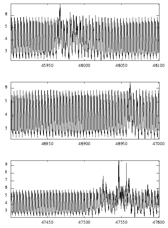
Analytic results about the asymptotic solutions of this equation, as well as some bifurcation results, can be found in [She '87]. More recently, interesting transitions that occur at higher Reynolds number have been studied in [She & Nicolaenko '90] and [Nicolaenko & She '91]. They lead to sparsely distributed bursts in time for a fairly large range of Reynolds number from a threshold of $Re \approx 20.5$ to $Re \approx 120$ (for k_f=8)⁴. The most striking feature of this transition is that the bursts generate substantial spatial disorder and drive developed turbulence. Typically, near threshold, the dynamics follow long laminar regimes, interspersed with chaotic bursts. Intervals between bursts are not constant and fluctuate randomly. We analyze this near-threshold dynamics here. Figure 6.21 illustrates this behavior. These plots are time series of the maximum magnitude of the convective term. Not plotted between the bursts are lengthy laminar regimes. One might theorize that these bursts can be explained by homoclinic or heteroclinic orbits in phase space, as was the case for the Kuramoto-Sivashinsky PDE in Section 6.1.1. Our goal is to compare laminar and burst data through a K-L analysis, looking for common spatial structures and trying to understand what is responsible for the bursting dynamics.

Figure 6.21 Intermittent bursts in Kolmogorov flow.

This example demonstrates how kltool can operate on various output data generated by the same PDE simulation. While the PDE numerical code integrates a stream function, turbulence theory prefers to deal with vorticity. We therefore analyze both stream and vorticity data, as well as the the Fourier amplitudes generated by the simulation. It should be noted that although vorticity is vector-valued, and kltool does not analyze vectors of vector-valued data, the x and y components of the vorticity are zero for 2D flow. Hence, the vorticity vector is strictly in the z-direction, and it is this component which is analyzed.

We mention a preprocessing step that was necessary before K-L analysis could proceed. For the Reynolds value of this example, the physical solution data is traveling in the x-direction. Theoretical analysis shows that the K-L eigenfunctions for a traveling wave become sinusoids. However, we are not interested in the analysis of the traveling wave, but want to treat it as one coherent structure, and study the remaining dynamics in the data. Hence, we process our data first, calculate the wave speed and go into a co-moving coordinate frame. We subtract the mean and perform our K-L analysis on the remaining data, both for the laminar and the bursting regime.

The simulation data come from a $64 \times 64$ pseudo spectral algorithm.

6.3.1. Stream Function Analysis

A K-L analysis on the laminar regime using the stream function data led to two eigenfunctions required for 95% of the total energy. These eigenfunctions are plotted in Figure 6.22.

Figure 6.22 Kolmogorov(stream, laminar): (89.8% of energy)(top) and (9.4% of energy)(bottom).

A reconstruction of the data using just those two modes together with the mean gives an almost perfect agreement between data and reconstruction. Using K-L on the Fourier amplitudes, we capture almost the same amount of energy in the first few eigenfunctions. Figure 6.23 shows the time series of coefficients for $\Psi_1$ and $\Psi_2$, indicating that they span a limit cycle.

Figure 6.23 Kolmogorov(stream, laminar): coefficients of and .

Analyzing the burst for the stream function data shows some surprising results. Here, three K-L modes are required to capture at least 95% of the energy. These are plotted in Figures 6.24 and 6.25. In addition, we show $\Psi_8$ in Figure 6.25 to illustrate how an eigenfunction, although containing very little energy, can contribute to localized spatial dynamics - at a vortex in this case.

Figure 6.24 Kolmogorov(stream, burst): (80.9% of energy)(top) and (12.1% of energy)(bottom).

Figure 6.25 Kolmogorov(stream, burst): (5.5% of energy)(top) and (0.1% of energy)(bottom).

The first mode, $\Psi_1$, in the laminar regime is roughly the same as $\Psi_1$in the bursting regime. However, both $\Psi_2$ and $\Psi_3$ in the bursting regime seem to be related to $\Psi_2$ in the laminar regime. It appears that they are real and imaginary parts of the same complex eigenfunction. This suggests that if a limit cycle lies in a real subspace, then its unstable manifold is in the imaginary subspace. This was corroborated by examining $\Psi_2$ and $\Psi_3$ in their Fourier representation.

6.3.2. Vorticity Analysis

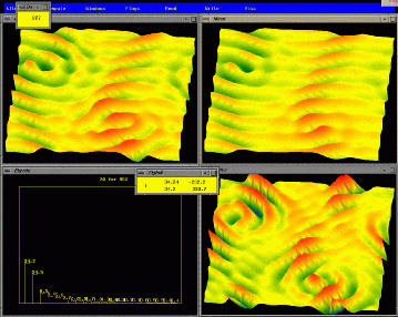
Figure 6.26 shows the results of analyzing the vorticity data in the laminar regime. Shown are: a snapshot vorticity vector (upper-left), the mean of the data (upper-right), the $\Psi$ energy percentages (lower-left), and $\Psi_1$(lower-right). The analysis indicates that five eigenfunctions are necessary to capture 95% of the energy.

Figure 6.26 Kolmogorov(vorticity, laminar): snapshot(u-l), mean(u-r), energy %s(l-l), (l-r).
(click on image for 1278x1022 enlargement)

In Figure 6.27, we show a different snapshot vorticity vector (upper-left) which highlights the eyes (vortices) in the eddies, and the $\Psi_2$ (lower-right). Notice that $\Psi_1$ contains the diagonal eddy structure, whereas $\Psi_2$ contains more of the vortices structure.

Figure 6.27 Kolmogorov(vorticity, laminar): snapshot(u-l), mean(u-r), energy %s(l-l), (l-r).
(click on image for 1278x1022 enlargement) Figure 6.28 shows the results of analyzing the vorticity data in the bursting regime. Shown are: a snapshot vorticity vector (upper-left), the mean of the data (upper-right), the $\Psi$ energy percentages (lower-left), and $\Psi_1$(lower-right). The analysis indicates that twenty eigenfunctions are necessary to capture at least 95% of the energy.

Figure 6.28 Kolmogorov(vorticity, burst): snapshot(u-l), mean(u-r), energy %s(l-l), (l-r).
(click on image for 1278x1022 enlargement)

In Figure 6.29, we show $\Psi_2$ (upper-left), $\Psi_3$ (upper-right), $\Psi_4$ (lower-left), and $\Psi_{11}$ (lower-right). Note that $\Psi_{11}$ is an especially localized vortex structure.

Figure 6.29 Kolmogorov(vorticity, burst): (u-l), (u-r), (l-l), (l-r).
(click on image for 1278x1022 enlargement) 6.3.3. Conclusions

We have not shown any reconstructions of the data using the eigenfunctions. This becomes difficult to do on paper when dealing with a sequence of 2D images. However, kltool lets a user synchronize the data vectors with the reconstructed vectors when scanning them. This technique, as well as scanning the error vectors, allows for a visual check of the reconstruction's accuracy to the data.

We concluded that the laminar regime is clearly a modulated traveling wave. Its wave speed can be calculated by observing the change in phase of a Fourier mode. In a coordinate frame moving with the traveling part, the oscillation is described by a limit cycle which is spanned by the first two eigenfunctions of the K-L decomposition for the stream function data. We independently confirmed this by extracting a scalar ``averaged'' quantity from the field (summing up a norm over a $16 \times 16$ grid in physical space). On the time series for that scalar quantity we performed a time-delay embedding and calculated the fractal dimension d_F [Kostelich & Swinney '89]. For both stream function and vorticity data we found d_F = 1.0.

There exists a low-dimensional large scale dynamics that drives the burst. We found that the unstable manifold of the laminar regime is very flat, concentrating the burst mainly along one dimension. This is again supported by plots of a time-delay embedding.

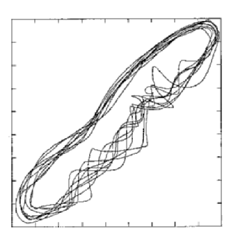
Figure 6.30 shows such a 2D time-delay plot. One sees the remnants of the basic limit cycle with faster oscillations superimposed. Computations of fractal dimensions suffer from too small a data set and are not very accurate. Initial calculations give d_F = 1.24 and d_F = 1.65for stream function and vorticity data, respectively. Both numbers are consistent with a K-L embedding dimension between 3 and 5 .

Figure 6.30 2D time-delay plot for an averaged scalar function of the vorticity field. One can distinguish a laminar dynamics following closely the original limit cycle and a faster, oscillatory phase with motion transverse to the limit cycle.

The biggest mystery of this analysis is the large discrepancy between the number of relevant eigenfunctions for stream function and vorticity data. From a dynamical systems point of view, if this system has a finite dimensional attractor then there exists only one dimension and all numbers for vorticity and stream function should agree with each other. However, the Laplacian obviously acts as a nonlinear weight function giving largest weight to the smallest scales of the PDE simulation. Therefore the general noise level of the vorticity data is increased up to a margin of about 5 % of the K-L energy. In order to check the dependence of the K-L results on the resolution of the PDE simulation, we enlarged our data set and used all Fourier modes available from the $64 \times 64$ pseudo spectral grid. The result is that we needed even more K-L eigenfunctions (25 versus 20) to capture 95% of the energy in the vorticity burst data. At the same time, visual inspection of the reconstruction was satisfactory with fewer K-L modes (10 modes versus 16). These results suggest that there are two types of dynamics going on during the burst phase: a large scale, low dimensional one which can be described by a structurally stable homoclinic orbit and which has very definite symmetry properties. This dynamics is best captured by looking at the behavior of the stream function. Riding on top of that dynamics is a small scale dynamics characterized by an enstrophy cascade: enstrophy is accumulating in the modes which are barely resolved and have the smallest scales. Better spatial resolution leads to an accumulation of enstrophy in the new, yet smaller scales.

For more details regarding the K-L analysis of the Kolmogorov flow, including a more in-depth discussion of how symmetries of the equation play an important role, see [Armbruster, Heiland, Kostelich & Nicolaenko '92]

6.4. Flame Dynamics

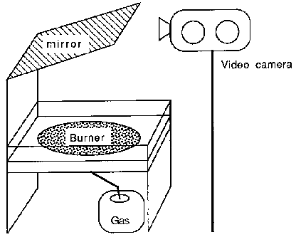
As a final example, we present an analysis of data from an experiment on the dynamics of two-dimensional flames [Gorman, el-Hamdi & Robbins '92]. A schematic of the experiment is shown in Figure 6.31.

Figure 6.31 Schematic illustration of flames experiment.

The apparatus consists of a flat, circular, porous plug burner which burns various premixed gases. A video camera records the resulting flame dynamics. Depending on the types of gases and their flow rate through the burner, one can observe fascinating spatiotemporal patterns of the flames. For example, one such pattern involves a stable rotating ring of flame cells about a central core of cells. The flames can become unstable due to a competition between thermal diffusivity and mass diffusivity resulting in some outer cells exchanging positions with some inner cells.

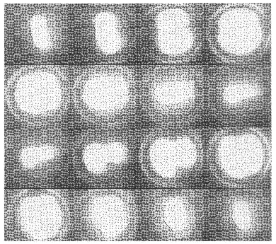
For input to kltool, we chose a simpler regime of flame dynamics to analyze. The flame in this regime was a single closed spatial structure which changed its shape in time. The first few video frames of the dynamics are shown in Figure 6.32.

Figure 6.32 First sixteen images of flame video data (left to right, top to bottom).
(click on image to see 821x726 enlargement)

We briefly describe the preprocessing steps involved in the analysis. First, the video images were digitized. Next, we subtracted the artifical reflective ring surrounding the flame. Upon analyzing these 2D images, the results were difficult to interpret. The eigenfunctions had to be mapped back into grayscale values for display and this resulted in confusing images. Realizing that what we actually wanted to analyze was the dynamics of just the boundary of the flame, we replaced the solid flame image with its boundary curve. This not only gave more meaningful results than working with the entire flame image, but also significantly decreased the computation time. The boundary curves are 1D spatial vectors: $r(\theta), 0\leq\theta\leq2\pi$, plotted in polar coordinates. They are shown superimposed on the flame images in Figure 6.32. Finding a flame boundary was straightforward for this particular regime. A parametrized radial sweep of a flame image yielded a unique intersection point with the flame edge (detected by a gradient change in light intensity).

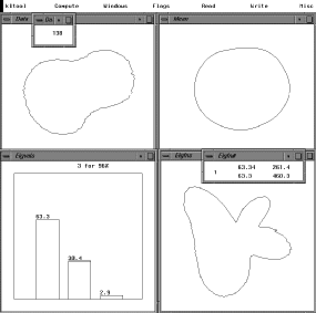
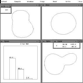
The resulting analysis by kltool is shown in Figures 6.33 and 6.34. Figure 6.33 shows a sample snapshot in the data window (upper-left), the mean (upper-right), the $\Psi$ energy percentages (lower-left), and $\Psi_1$(lower-right). The analysis indicates that only two K-L modes are responsible for most of the dynamics. Notice that $\Psi_1$, the primary coherent structure, is quadrapole-shaped. Figure 6.34 shows a different snapshot (upper-left) and a dipole-shaped $\Psi_2$ (lower-right).

Figure 6.33 Flames: snapshot(u-l), mean(u-r), energy %s(l-l), (l-r).
(click on image to see 825x819 enlargement)

Figure 6.34 Flames: snapshot(u-l), mean(u-r), energy %s(l-l), (l-r).
(click on image to see 825x819 enlargement)

In Figure 6.35, we plot the time series of coefficients for $\Psi_1$ and $\Psi_2$. Their oscillatory behavior clearly indicates that we have a limit cycle which is spanned by these first two K-L modes.

7. Future Directions

There are at least two parallel directions for the future of kltool. In one direction, we forsee added functionality. For example, since the tool currently allows for the visualization of only one- and two-dimensional spatial vectors, an obvious extension would be the visualization of trivariate data. This seemingly insignificant increase by one dimension has a significant impact on the computational cost, as well as the visualization challenge. One could alleviate these problems by running the tool on a dual-platform. The lengthy computations could be performed on a more powerful processor, then the results displayed on the graphical workstation. Regarding the computational issue, we note that a parallel processor would be very efficient for computing the covariance matrix. Another extension in functionality would be to analyze vectors of vector values instead of vectors of scalar values. Additional functionality might be to compute eigenfunctions which have different optimality criteria. Such an approach is discussed in [Kirby '92]. An addition to the Galërkin projection would be to allow for numerical integration of the ODEs and display the resulting trajectories.

The second direction for the future of kltool is to broaden its accessibility. The primary limitation at this time is its dependence on the Silicon Graphics workstation and the Graphics Library. One could rewrite the graphics-dependent software for other computers, taking advantage of available hardware, and thereby offer a larger set of platforms on which the tool could run. However, a more likely option would be to write the graphics-dependent software in a standard graphics application language. Although the Graphics Library itself has been ported to other computers, the apparent standard package for graphics applications is the X library [Nye '88]. Unfortunately, at the present time, the 3D graphics in the X library does not seem to be well established.

8. Summary

An interactive graphical software package, kltool, has been presented for the analysis of spatiotemporal data. The tool uses the Karhunen-Loève (K-L) decomposition to compute empirical eigenfunctions which optimally span a given dataset. These eigenfunctions, $\Psi_i$, can indicate coherent spatial structures within the data. By projecting the data onto the $\Psi_i$, it is possible to gain a better understanding of their temporal dynamics within a dynamical systems framework. Through this analysis, one can gain insight into the asymptotic behavior of a given system and can get an estimate on the dimension of an underlying attractor.

We have demonstrated kltool's effectiveness on four different example datasets: two from PDE simulations and two from laboratory experiments. For particular regimes of the Kuramoto-Sivashinsky (K-S) and Kolmogorov PDEs, we showed how certain eigenfunctions (K-L modes) correspond to fixed points and how others span limit cycles. We also showed how certain K-L modes are responsible for bursting behavior. A Galërkin projection was automatically generated for the K-S PDE using three eigenfunctions. The analysis of the Couette-Taylor experimental data indicated rather complex dynamics. It would be interesting to have more data of this type for further analysis. The gas flame dynamics seemed to be evolving on a limit cycle spanned by two K-L modes.

We do not wish to leave the impression that this tool will always provide a simple analysis of any spatiotemporal dataset. However, if used wisely, we feel that it can benefit many researchers investigating nonlinear systems.

Bibliography

Abraham, R.H. and Shaw, C.D. (1984), Dynamics: The Geometry of Behavior, Ariel Press, Santa Cruz.

Armbruster, D., Guckenheimer, J. and Holmes, P. (1989), Kuramoto-Sivashinsky dynamics on the center-unstable manifold, SIAM J. Appl. Math. 49, 676-691.

Armbruster, D. and Heiland, R. (1992), kltool: User's Manual. Dept. Mathematics, Arizona State University, Tempe.

Armbruster, D., Heiland, R., Kostelich, E.J. and Nicolaenko, B. (1991), Phase space analysis of bursting behavior in Kolmogorov flow, to appear in Physica D.

Aubry, N., Holmes, P., Lumley, J.L. and Stone, E. (1988), The dynamics of coherent structures in the wall region of a turbulent boundary layer, J. Fluid Mech. 192, 115-173.

Barnsley, M.F. (1988), Fractals Everywhere, Academic Press, London, 172-199.

Broomhead, D.S. and King, G.P. (1986), Extracting qualitative dynamics from experimental data, Physica 20D, 217-236.

Chorin, A.J. and Marsden, J.E. (1990), A Mathematical Introduction to Fluid Mechanics, Springer-Verlag, New York, 32-46.

Crawford, J.D. (1991), Introduction to bifurcation theory, Rev. Modern Physics 63, 991-1037.

DiPrima, R.C. and Swinney, H.L. (1981), Instabilities and transition in flow between concentric rotating cylinders, in: Swinney, H.L. and Gollub, J.P., eds., Hydrodynamic Instabilities and the Transition to Turbulence, Springer-Verlag, New York, 139-180.

Eckmann, J.P. (1981), Roads to turbulence in dissipative dynamical systems, Rev. Modern Physics 53, 643-654.

Farmer, J.D., Ott, E. and Yorke, J.A. (1983), The dimension of chaotic attractors, Physica 7D, 153-180.

Fukunaga, K. (1990), Introduction to Statistical Pattern Recognition, Academic Press, San Diego.

Gibson, J.F., Farmer, J.D., Casdagli, M. and Eubank, S. (1992), An analytic approach to practical state space reconstruction, Santa Fe Institute report #92-04-021.

Gleick, J (1987), Chaos: Making a New Science, Viking Press, New York.

Gonzalez, R.C. and Wintz, P. (1987), Digital Image Processing, 2nd Edition, Addison-Wesley, Reading, MA, 122-130.

Gorman, M., el-Hamdi, M. and Robbins, K.A. (1992), Spatiotemporal chaotic dynamics of premixed flames, in: Vohra, S., Spano, M., Shlesinger, M., Pecora, L. and Ditto, W., eds., Proceedings of the 1st Experimental Chaos Conference, World Scientific, Singapore, 403-416.

Guckenheimer, J. and Holmes, P. (1983), Nonlinear Oscillations, Dynamical Systems, and Bifurcations of Vector Fields, Springer-Verlag, New York.

Guckenheimer, J. and Kim, S. (1990), kaos: Dynamical Systems Toolkit with Interactive Graphics Interface Mathematics Dept., Cornell University.

Hirsch, M.W. and Smale, S. (1974), Differential Equations, Dynamical Systems, and Linear Algebra, Academic Press, Orlando.

Hyman, J.M., Nicolaenko, B. and Zaleski, S. (1986), Order and complexity in the Kuramoto-Sivashinsky model of weakly turbulent interfaces, Physica 23D, 265-292.

Jolly, M.S, Kevrekidis, I.G. and Titi, E.S. (1990), Approximate inertial manifolds for the Kuramoto-Sivashinsky equation: analysis and computations, Physica 44D, 38-60.

Kevrekidis, I.G., Nicolaenko, B. and Scovel, J.C. (1990), Back in the saddle again: A computer assisted study of the Kuramoto-Sivashinsky equation, SIAM J. Appl. Math. 50, 760-790.

Kirby, M. (1992), Minimal dynamical systems from PDEs using Sobolev eigenfunctions, to appear in Physica D.

Kirby, M. and Armbruster, D. (1991), Reconstructing phase space for PDE simulations, to appear in ZAMP.

Koçak, H. (1986), Differential and Difference Equations through Computer Experiments, Springer-Verlag, New York.

Kostelich, E.J. (1992) Problems in estimating dynamics from data, to appear in Physica D.

Kostelich, E.J. and Swinney, H.L. (1989), Practical considerations in estimating dimension from time series data, Physica Scripta 40, 436-441.

Kostelich, E.J. and Yorke, J.A. (1990), Noise reduction: Finding the simplest dynamical system consistent with the data, Physica 41D, 183-196.

Libchaber, A., Fauve, S. and Laroche, C. (1983), Two-parameter study of the routes to chaos, Physica 7D, 73-84.

Lorenz, E.N. (1963), Deterministic non-periodic flow, J. Atmos. Sci. 20, 130-141.

Lumley, J.L. (1967), Atmospheric Turbulence and Radio Wave Propagation, Yaglom, A.M. and Tatarski, V.I., eds., Nauka, Moscow, 166-.

Mees, A.I., Rapp, P.E. and Jennings, L.S. (1987), Singular-value decomposition and embedding dimension, Physical Rev. A 36, 340-346.

Newell, A.C. and Moloney, J.V. (1992), Nonlinear Optics, Addison-Wesley, Redwood City, CA.

Newell, A.C., Rand, D.A. and Russell, D. (1988), Turbulent transport and the random occurrence of coherent events, Physica 33D, 281-303.

Nicolaenko, B. and She, Z.S. (1991), Symmetry breaking homoclinic chaos and vorticity bursts in periodic Navier-Stokes flows, Eur. J. Mech., B/Fluids 10, 67-74.

Nye, A. (1988), Xlib Programming Manual, O'Reilly & Associates, Inc., Sebastopol, CA.

Rodriguez, J.D. and Sirovich, L. (1990), Low-dimensional dynamics for the complex Ginzburg-Landau equation, Physica 43D, 77-86.

Roux, J.-C. (1983), Experimental studies of bifurcations leading to chaos in the Belousof-Zhabotinsky reaction, Physica 7D, 57-68.

Ruelle, D. (1989), Chaotic Evolution and Strange Attractors, Cambridge University Press, Cambridge, England, 23-27.

Ruelle, D. (1991), Chance and Chaos, Princeton University Press, Princeton, NJ, 51-65.

Sauer, T., Yorke, J.A. and Casdagli, M. (1991), Embedology, J. Statist. Phys. 65, 579-616.

She, Z.S. (1987), Metastability and vortex pairing in Kolmogorov flow, Phys. Lett. A 124, 161-164.

She, Z.S. and Nicolaenko, B. (1990), Temporal intermittancy and turbulence production in the Kolmogorov flow, in: Moffatt, H.K., ed., Topological Fluid Mechanics, Cambridge University Press, Cambridge, England.

Shneiderman, B. (1980), Software Psychology, Little, Brown and Co., Boston, 216-266.

Sirovich, L. (1987a), Turbulence and the dynamics of coherent structures, Part I: Coherent Structures, Quarterly of Appl. Math. XLV, 561-571.

Sirovich, L. (1987b), Turbulence and the dynamics of coherent structures, Part III: Dynamics and Scaling, Quarterly of Appl. Math. XLV, 583-590.

Sirovich, L. and Kirby, M. (1987), Low-dimensional procedure for the characterization of human faces, J. Opt. Soc. Am. A 4, 519-524.

Sparrow, C. (1982), The Lorenz Equations, Springer-Verlag, New York.

Stewart, I. and Golubitsky, M. (1992), Fearful Symmetry, Blackwell, Cambridge, MA, 104-118.

Stone, E. (1992), Bifurcation structures of minimal ODEs from weighted Sobolev projections of PDEs, in: Proceedings of Conference on Bifurcations and Symmetries, SIAM AMS Summer Workshop, Ft. Collins, CO.

Strang, G. (1976), Linear Algebra and its Applications, Academic Press, New York.

Strang, G. (1986), Introduction to Applied Mathematics, Wellesley-Cambridge Press, Wellesley, MA.

Sugihara, G. and May, R.M. (1990), Nonlinear forecasting as a way of distinquishing chaos from measurement error in time series, Nature 344, 734-741.

Swinney, H.L. (1984), Observations of complex dynamics and chaos, in: Cohen, E.G.D., ed., Fundamental Problems in Statistical Mechanics VI, North-Holland, Amsterdam.

Takens, F. (1981), Detecting strange attractors in turbulence, in: Rand, D.A. and Young, L.-S., eds., Dynamical Systems and Turbulence, Lecture Notes in Math. 898, Springer-Verlag, New York, 366-381.

Waltman, P. (1986), A Second Course in Elementary Differential Equations, Academic Press, New York.

Wiggins, S. (1988), Global Bifurcations and Chaos, Springer-Verlag, New York.

Wiggins, S. (1990), Introduction to Applied Nonlinear Dynamical Systems and Chaos, Springer-Verlag, New York.

Yorke, J. (1990), Dynamics: A Program for IBM PC Clones, Depart. Mathematics, University of Maryland, College Park.

Appendix A

Galërkin Projection for Kuramoto-Sivashinsky PDE

This appendix accompanies the analysis in Section 6.1.1. The input file specifying the K-S PDE, which will be parsed by kltool, is the following:

u(t,x) 
# This file provides the Kuramoto-Sivashinsky PDE
# in the desired syntax for parsing by kltool.
# The first line of the file specifies the dependent function
# and independent variables.
#
# d(u,t) = 
 -4*d(u,x,4) - alpha * ( d(u,x,2) + 0.5*d(u,x)^2 )

The following is the resulting Galërkin projection, a system of ODEs, obtained from the first three K-L modes:

a1 * 4.77502174e-01 =  -  4  * 
 ( a1 * 7.64229734e+00  + a2 * -1.30090583e-01  + a3 * 8.35663964e-02  )  
 -  alpha  *  ( 
 ( a1 * -1.90954685e+00  + a2 * 2.70510994e-02  + a3 * -1.68602983e-02  )  
 +  0.5  * 
 ( a1*a1 * 1.46427749e-02 + a1*a2 * -3.82984342e-03 + a1*a3 * -4.23164926e-02 
 + a2*a1 * -3.82984342e-03 + a2*a2 * -2.42889080e-04 + a2*a3 * -2.24138759e-01 
 + a3*a1 * -4.23164926e-02 + a3*a2 * -2.24138759e-01 + a3*a3 * 9.23985816e-03 ))




a2 * 5.21931895e-01 =  -  4  * 
 ( a1 * -1.30090583e-01  + a2 * 5.43366793e-01  + a3 * 3.00340148e-04  )  
 -  alpha  *  ( 
 ( a1 * 2.70510994e-02  + a2 * -5.24061964e-01  + a3 * 1.73820964e-04  )  
 +  0.5  * 
 ( a1*a1 * -9.71341170e-03 + a1*a2 * 1.04331524e-02 + a1*a3 * 5.34356186e-01 
 + a2*a1 * 1.04331524e-02 + a2*a2 * -2.16584341e-04 + a2*a3 * -8.41680678e-03 
 + a3*a1 * 5.34356186e-01 + a3*a2 * -8.41680678e-03 + a3*a3 * 1.24558107e-02 )) 



a3 * 5.26295447e-01 =  -  4  * 
 ( a1 * 8.35663964e-02  + a2 * 3.00340148e-04  + a3 * 6.41147474e-01  )  
 -  alpha  *  ( 
 ( a1 * -1.68602983e-02  + a2 * 1.73820964e-04  + a3 * -5.33260817e-01  )  
 +  0.5  * 
 ( a1*a1 * 3.11884903e-02 + a1*a2 * 5.28333621e-01 + a1*a3 * -9.22197842e-03 
 + a2*a1 * 5.28333621e-01 + a2*a2 * -3.38895660e-02 + a2*a3 * 3.73078284e-03 
 + a3*a1 * -9.22197842e-03 + a3*a2 * 3.73078284e-03 + a3*a3 * -1.90138218e-02 ))

These equations represent $d{\bf a}/dt$. The user would need to divide each equation by the constant on the left-hand side before inserting the system into a numerical ODE solver.

 

• About this document ...